This is a writeup of my recent challenge for Imaginary CTF called Complex Curve Crypto.
 1from sage.all import *
 2phi = classical_modular_polynomial(l:=3)
 3flag = ZZ.from_bytes(os.environ.get('FLAG', 'jctf{fakeflag}').encode())
 4j = jp = ComplexField(1337)(1337)
 5for d in flag.digits(l):
 6    roots = phi(X=j).univariate_polynomial().roots(multiplicities=False)
 7    roots.sort(key=jp.dist)
 8    del roots[0] # no turning back
 9    roots.sort(key=arg)
10    j, jp = roots[d], j
11print(j)
12# -6380.29156755903034687704660000282270448709570700984709657263854520138341881550084848649839410922876936678108641559731906139407589458824525200739437427675429842545943862350406898342718600643307574207936681432539822432021043321858999100455988010088297166788530685045590301521392833041157761230553808660966639987227996254364651040683587985017755013287627806460764447918220597797227073500295101888328945378 - 40214.6672669145274363733990190234269396915010860735171342583778810557492152506583335099397606096949655915384682940536670398063862158837139959936293817852537495478495004482851179789975853315750442943613549504080182872285152393975211173312274904654221951964258004673123691758298620284682558712820558193891787303533093197420998108945366704043133890680849252774739771188873183182185315971489373696493547256*I
The last line there is the output of the script when it was ran with the real flag as input, which we have to use to somehow recover the flag.
The majority of this post is about explaining some of the machinery behind the solution, even though it’s not strictly needed to solve.
Isomorphism to Complex Tori
The unit circle
Here we will be drawing many parallels between the paramaterization of elliptic curves and the unit circle. There will be some handwaving and basically no proper proofs, what I aim to deliver is some intuition.
The defining equation of the unit circle is
We can parameterize the unit circle by
and you can verify that for any angle we have according to the Pythagorean identity.
In fact, is the general solution of the differential equation , which suggests that this is a kind of “natural” parameterization.

This parameterization is periodic with a period of , since
for all .
We can define a group on the unit circle by defining a binary operation
which simply sums angles. Now because , is ambigous for a given point up to integer multiples of , i.e up to elements of . We can explicitly encode this ambiguity as a quotient group which tells us that, with respect to the group operation , ; the real numbers modulo .
An elliptic curve
A general elliptic curve over can, after a change of variables, be written in short Weierstrass form:
Drawing from the previous section, it’s natural to ask if there is a similar parameterization of elliptic curves, perhaps one which also arises from a differential equation. Indeed, there is such a parameterization, which is given by the Weierstrass function, defined over .
Due to historical reasons it is a solution to the differential equation
where and define the shape of the curve. We can use this to parameterize our familiar short Weierstrass form by letting which satisfies the equation
which aligns with our definition of above if we let and . So to be clear, there is not one Weierstrass function, but rather a family of them, parameterized by the coefficients and . If they are evident from the context we often omit these parameters, otherwise we write .
An important property of is that it is doubly periodic. is, over the complex plane, only a singly periodic function; it repeats along the real axis, but not along the imaginary axis.
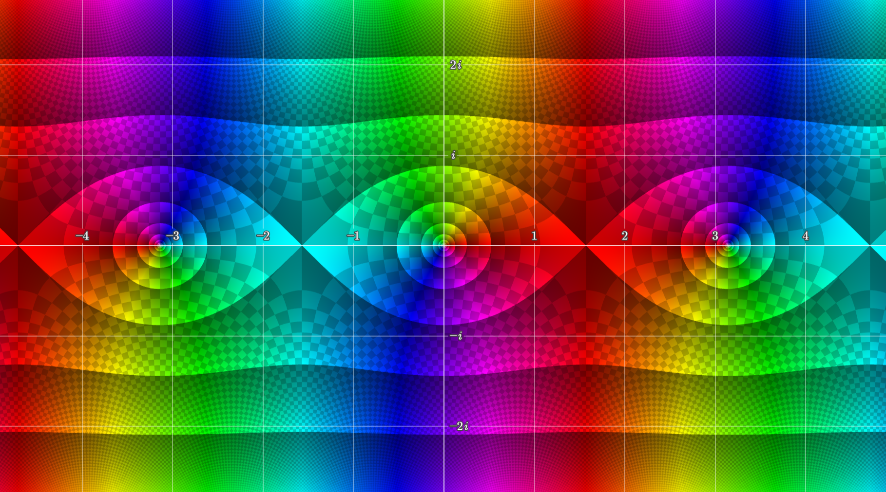
plotted over using Samuel J. Li’s complex function plotter.
on the other hand has two different periods, . is invariant under all integer linear combinations of these two periods, i.e for the lattice spanned by and
it holds that
For example, in the below figure we can make out the lattice points at which the function repeats.
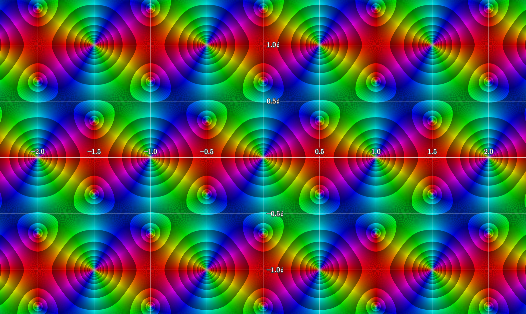
with plotted over using Samuel J. Li’s complex function plotter
The extremely important and cool property of is that addition (in the normal -sense) of the input parameters corresponds to addition of elliptic curve points, i.e
By a similar argument to previously, since is ambigous up to elements of , we can with some handwaving conclude that , also known as a complex torus.
The modulus
We say that two complex lattices and are homothetic if there exists some such that . This means that they are equivalent up to a scaling factor, and it is equivalent with (proof as per usual omitted). This should not be very surprising; multiplication by a complex number is equivalent to a scaling and a rotation which does not meaningfully change the shape of the lattice.
We will only be interested in lattices up to homothety, we can therefore rescale a lattice basis by to obtain a new basis where . By convention we restrict ourselves to , if that is not the case we can instead rescale by . This lets us represent this basis by a single number , which we call the modulus, which is part of the upper half plane .
The modulus is however not invariant under choice of basis for , let’s try to properly describe this.
If a lattice is defined by a basis then we can describe a change-of-basis by a matrix
A classical result stemming from ordinary lattices in implies that this new basis spans the same lattice if and only if and , which means , the general linear group over .
After this transformation we can then homothetically rescale by to get back to our simplified form with . With this transformation in mind we define the action of a matrix on as
This is known as a Möbius transformation. As concluded previously the new lattice is only homothetic if . We further restrict ourselves to to avoid becoming negative, which means that , the special linear group over .
Furthermore , so we can quotient out by this ambiguity and consider to be in , also known as the modular group.
We can therfore finally say that is defined up to the left action of on , in other words .
The j-invariant
If you are used to working with elliptic curves you might know that the -invariant of an elliptic curve with short Weierstrass coefficients is given by
and that if two elliptic curves and are isomorphic then they neccesarily have the same -invariant, i.e . Over an algebraically closed field like this is an equivalence, i.e
Going back to complex lattices, the -invariant can similarly be defined as function which is invariant under the action of on , which as we remember is the same as homothety of lattices, which is the same as isomorphism of elliptic curves. Since we have classified the ambiguity of this is actually a bijection if we modify the domain to be , i.e
You might have heard the term modular function before, and in fact this invariance under the modular group (together with some other properties) makes into a modular function of weight , but we won’t go down that rabbit hole here.
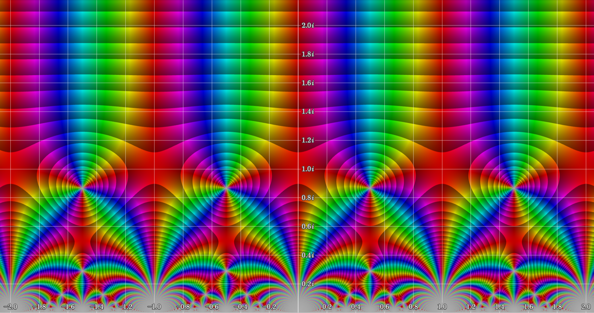
plotted over using Samuel J. Li’s complex function plotter. Notice the many different symmetries.
Isogenies
I won’t recap the definition of an isogeny here. The important thing to know is that an isogeny is a map between two elliptic curves which is a group homomorphism:
The degree of an isogeny is the size of the kernel and is a finite subgroup of , so an isogeny of degree is is simply an isomorphism because has to be in the kernel.
Let’s restrict ourselves to being prime. Then if we have that is a cyclic subgroup of , and more specifically : the -torsion subgroup of which consist of all points such that .
If we let be the lattice associated with then corresponds to points such that , more precisely
You might have seen this stated for elliptic curves over finite fields, this is really where that comes from. Let’s represent each point in by according to the above construction. Then we can describe a cyclic subgroup by a generator . Notice however that multiple generators can generate the same subgroup, since for , we therefore need to classify these subgroups up to scaling.
We do this by quotienting out by the relation , which yields
which is the projective line over the ring . The size of this set is for prime , and more generally it is where is the Dedekind psi function. What this all tells us is that there are distinct cyclic subgroups of , and thus distinct cyclic isogenies of degree from . Furthermore the generator of the kernel looks like for and as described above.
For prime we have that
So what does this tell us about the codomain of , i.e the curve and its lattice ? One can show that , when defined as a map between the complex tori, is a complex linear map of the form for some . Since this is a group homomorphism we must have that , which means that all points of must be mapped to points of . As a consequence we have that . Furthermore we have specified a subgroup which should also be mapped to , we must therefore also have that our kernel, generated by , is mapped to . All in all this means the full set of kernel points is generated by . We can reduce this to only two generators, with two different cases:
The second case is from rescaling by . With some handwaving we conclude that this will be homothetic to the lattice of the codomain, . Written in terms of matrices and Möbius transformations we have that
where is the set of matrices which correspond to the transformations above:
The challenge
The challenge, in a somewhat obscured way, is performing an isogeny walk starting from and choosing each next step based on the contents of the flag. The goal is thus to find the path between the given and .
The program uses a classsical modular polynomial to achieve this. A classical modular polynomial is a symmetric polynomial such that if and only if there exists a cyclic isogeny of degree between the elliptic curves with -invariants and . We can thus find curves which are -isogenous to a given -invariant by finding the roots of the univariate polynomial . This univariate polynomial has degree , which aligns with our findings previously that there should be distinct cyclic isogenies of degree from a given elliptic curve.
Based on the previous section, what do we know about the relation between and ? We have talked a lot about the action of isogenies on their corresponding lattices, so let’s start by calculating them.
You can do this manually using some complex AGM shenanigans, but since the year is 2025 it is already implemented in SageMath (make sure to use a recent version, otherwise .period_lattice() won’t be implemented for general fields).
1sage: j0 = CC(1337)
2sage: EllipticCurve(j=j0).period_lattice().tau()
30.131756389015516 + 0.991282126316011*I
This gives us exactly the we have been working with from before. Recall however that is ambigous for a given -invariant up to action of Möbius transformations of . Let’s take to be canonical. Then we have that for some integer matrix . More specifically, it is a sequence of isogenies, i.e matrices from from before, and finally a transformation which accounts for the ambiguity of the final . We can thus write
where is the number of base digits in the flag. We want to recover the matrix of this transformation. Per definition of the Möbius transformation we have that
This is a linear equation in the variables which we want to find a close solution to (due to precision issues it won’t be exact). Since they are complex numbers this becomes two real-valued equations, saying that both the imaginary and real part should be zero. This is a perfect application of lattice reduction, let’s therefore reduce the lattice spanned by the rows of the following matrix
Where is sufficiently large, works since is the bit-precision of the given numbers. We thereby hope to find the following vector
Which works. There are now (at least) two different ways to proceed.
Simple method: Determinant search
Let’s calculate the determinant of the recovered transformation:
This means that we can tell at any given -invariant how far away we are from by calculating the determinant of this transform. From there you can simply try all neighbors of and check if they get closer or further away from . Repeating this you can walk backwards and recover the path of -invariants, which yields the flag digits.
Less simple method: Factor the transformation
I thought it would be fun to try and factor the transformation directly, without using the -invariants for guidance. I am however too lazy to write this up, so I will just leave the code here in case anyone is interested in understanding it.
 1from sage.all import *
 2from sage.geometry.hyperbolic_space.hyperbolic_isometry import moebius_transform
 3
 4def normalize_Sn(M):
 5    # make upper-triangular
 6    c, d = matrix([[M[0,0], M[1,0]]]).right_kernel_matrix()[0]
 7    g, a, b = xgcd(d, -c)
 8    assert g == 1
 9    M = matrix([[a, b], [c, d]]) * M
10
11    # positive diagonal
12    assert M[0,0].sign() == M[1,1].sign()
13    if M[0,0] < 0:
14        M = -M
15
16    # make 0 <= b < d
17    M[0, 1] %= M[1, 1]
18    return M
19
20def product_candidates(M, pathlen, path=()):
21    M = M.change_ring(ZZ)
22    if M.is_one():
23        yield path
24        return
25    if len(path) == pathlen:
26        return
27
28    if M[0, 0] % l == M[0, 1] % l == 0:
29        T = matrix([[l, 0], [0, 1]])
30        yield from product_candidates(T**-1*M, pathlen, path + (T,))
31
32    if M[1, 1] % l == 0:
33        b = M[0,1]//(M[1,1]//l)
34        T = matrix([[1, b], [0, l]])
35        yield from product_candidates(T**-1*M, pathlen, path + (T,))
36
37def inv_j(j):
38    return EllipticCurve(j=j).period_lattice().tau()
39
40C = ComplexField(prec:=1337)
41j0 = C(1337)
42j = C('...') # the given output
43
44phi = classical_modular_polynomial(l:=3)
45tau0, tauA = inv_j(j0), inv_j(j)
46
47M = matrix([[tau0, 1, -tau0*tauA, -tauA]]).T
48L = (M.apply_map(real)
49     .augment(M.apply_map(imag))
50     .change_ring(QQ)*2**prec).augment(identity_matrix(M.nrows()))
51M = matrix(ZZ, 2, 2, L.LLL()[0][2:])
52ndig = M.det().valuation(l)
53assert M.det() == l**ndig
54
55for path in product_candidates(normalize_Sn(M), ndig):
56    digits = []
57    j, tau = j0, tau0
58    jp = j
59    for mat in path[::-1]:
60        roots = phi(X=j).univariate_polynomial().roots(multiplicities=False)
61        roots.sort(key=jp.dist)
62        del roots[0]
63        roots.sort(key=arg)
64
65        tau = moebius_transform(mat, tau)
66        j, jp = elliptic_j(tau), j
67        d = min(range(len(roots)), key=lambda i: j.dist(roots[i]))
68        digits.append(d)
69    print(ZZ(digits, l).to_bytes(32).lstrip(b'\x00').decode())