Matrix multiplication over $\mathbb{F}_2$ using M4RM and AlphaTensor

The field with two elements, $\mathbb{F}_2$, is both very useful in the context of bit operations on computers, but also therefore extremely fast to compute in. Addition is XOR and multiplication is AND, both of which are native intructions on basically all architectures.

In this post I’ll explain the state-of-the-art techniques used to multiply matrices in over $\mathbb{F}_2$, which I learned about when implementing them myself in Rust as a personal project here.

At least on my computer I managed to reach and sometimes surpass the performance of the 🐐 M4RI, and I think this is the first time that the modular algorithms discovered by Google DeepMind’s AlphaTensor is implemented in an otherwise state-of-the-art $\mathbb{F}_2$ matrix multiplication library.

Though I may just have overfitted parameters to my own computer and it’s actually quite mid, feel free to benchmark yourself.

The Method of the Four Russians

This explanation is very similar to the one in Efficient Multiplication of Dense Matrices over GF(2) by the M4RI authors, which is what I used to understand the algorithm myself.

The algorithm was introduced by V. L. Arlazarov, E. A. Dinic, M. A. Kronrod, and I. A. Faradžev, and the name is explained by Aho, Hopcroft & Ullman in The Design and Analysis of Computer Algorithms:

The second method, often called the “Four Russians’” algorithm, after the cardinality and nationality of its inventors, is somewhat more “practical” than the algorithm in Theorem 6.9.

It is also the origin of M4RI’s name.

The core idea of the algorithm is to precompute linear combinations which we might need later, and we then hope that many of the linear combinations can be reused thus saving us time.

Outer products

You might be used to thinking of the matrix product $\mathbf{C} = \mathbf{A B}$ as computing inner products between each of the rows of $\mathbf{A}$ with each of the columns of $\mathbf{B}$, and putting them in their respective entries in $\mathbf{C}$. There is however many different ways to look at it, and one of them is as a sum of outer products between columns of $\mathbf{A}$ and rows of $\mathbf{B}$.

Let $\mathbf{A} \in \mathbb{F}_2^{m \times k}$ and $\mathbf{B} \in \mathbb{F}_2^{k \times n}$ . Let’s borrow some Python syntax and let ${\mathbf{A}[:,i]} \in \mathbb{F}_2^{m \times 1}$ denote the $i$th column of $\mathbf{A}$ and ${\mathbf{B}[i, :]} \in \mathbb{F}_2^{1 \times n}$ denote the $i$th row of $\mathbf{B}$, then we have that ${\mathbf{A}[:, i] \mathbf{B}[i, :]} \in \mathbb{F}_2^{m \times n}$, and we can write the matrix product as

But we don’t need to slice things up into just $1$ wide slices, let’s instead fix a slice-width $s$ and let’s for simplicity assume that $s | k$. Once again using Python syntax, we then have that

Slice multiplication

The key now comes in how we compute each of these products of a slice ${\mathbf{A}[:, is : (i+1)s]} \in \mathbb{F}_2^{m \times s}$ and ${\mathbf{B}[is : (i+1)s, :]} \in \mathbb{F}_2^{s \times n}$. Let’s consider the example of $m=3, n=4, s=2$. Let’s denote the slice of $\mathbf{A}$ as $\mathbf{A}_i$ and the slice of $\mathbf{B}$ as $\mathbf{B}_i$, and let

A way to compute the $m \times n$ product $\mathbf{A}_i \mathbf{B}_i$ is to look at each row of $\mathbf{A}_i$ and multiply to the left of $\mathbf{B}_i$, effectively selecting a linear combination of the rows of $\mathbf{B}_i$. Each result is then put in the next row of the result matrix.

So each row of the result is some linear combination of the rows of $\mathbf{B}_i$.

These are exactly the linear combinations which we precompute and save in a table, when $m$ is sufficiently large this can save us a lot of time.

Gray codes

So we want to compute all possible linear combinations of the rows of $\mathbf{B}_i$. Since we are in $\mathbb{F}_2$ there are $2^s$ possible linear combinations, we either select each row or we don’t, and then we sum them all together.

The Gray Code is a way to order the binary numbers such that two consecutive numbers differ only in one bit position. The Gray Code for $3$ bits looks like this

Let’s consider the Gray Code for $s$ bits, and let’s imagine that each bit position in the code corresponds to the coefficient of a row in $\mathbf{B}_i$. Basically each of these sequences of $s$ bits is a possible row of $\mathbf{A}_i$.

The powerful thing about this is that in order to get from one code to the next we only need to change one bit, which corresponds to a single row addition from $\mathbf{B}_i$. Thus, to compute the entire table we only need to perform $2^s-1$ row additions, as opposed to roughly $(k/2-1)2^k - 1$ if we computed each one separately.

In M4RI $s$ is chosen dynamically based on the size of the matrices involved, in my implementation I fix $s=8$ which simplifies the implementation a bit since each row of $\mathbf{A}_i$ will be a single byte. Apparently it doesn’t degrade performance much either.

The actual implementation is not that large and is mostly self-contained in this file.

AlphaTensor

In 2022 Google’s DeepMind team released their research on matrix multiplications viewed as a reinforcement learning problem, known as AlphaTensor. They focused on finding ways of computing products of block matrices (i.e matrices of matrices) which uses as few multiplications as possible.

The most well-known algorithm for this is the Strassen algorithm, which uses $7$ multiplications instead of the naive $8$ to multiply two $2 \times 2$ matrices. This has been proven optimal, and only the number of additions has been reduced since.

The AlphaTensor team managed to improve upon the best-known algorithms for several other matrix sizes, and convenientely they also searched for algorithms which specifically work in $\mathbb{F}_2$ but not neccessarily in $\mathbb{R}$. They managed to find an algorithm for multiplying two $4 \times 4$ matrices using $47$ multiplications instead of $49$ (which is what you get if you chain $2 \times 2$ multiplications). They also improved $5 \times 5$ multiplication, down to $96$ multiplications instead of the previously best-known $98$. These are arguably not huge improvements, but for large matrices I found that they did make a noticeable difference.

From what I’ve read the results for $\mathbb{F}_2$ where largely seen as a curiosity (I guess the ML community doesn’t care abour $\mathbb{F}_2$ as much as I do ), so I decided to implement them here to see what kinds of performance gains they could give.

Results

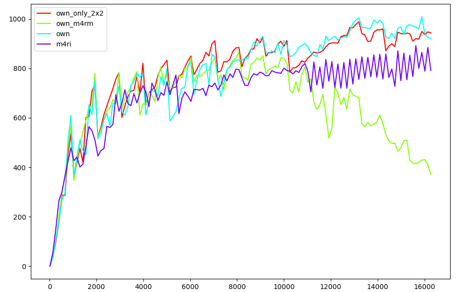
Here are some performance graphs comparing:

• own_only_2x2: My own implementation, using only $2 \times 2$ block multiplications.
• own_m4rm: My own implementation, without any block multiplications.
• own: My own implementation, using both $2 \times 2$ and $4 \times 4$ block multiplications.
• m4ri: The M4RI library.

The $x$-axis is the dimension of two square matrices that are being multiplied. The $y$-axis is $x^3/c$ where $c$ is the number of CPU cycles that it took to compute the product, i.e higher on the $y$-axis is better. This roughly measures bit-operations per cycle.

Conclusions

It’s interesting to see the dip in performance of non-blocked multiplication at around the $11000$ mark. This corresponds quite well to where the two matrices can no longer fit in my L3 cache. It is 32 MiB, each matrix gets half of that, which would correspond to a square matrix of dimension $\sqrt{8 \cdot 32 \cdot 1024^2 / 2} \approx 11585$, so close enough in my opinion.

You’ll notice that I didn’t use e.g $5 \times 5$ block matrix multiplication. This is largely a skill issue, finding how to optimally decompose a given matrix size into differnet recursive block sizes turned out to be non-trivial, at least for me. I might go back and implement it in the future.

Furthermore the advantage of using $4 \times 4$ block multiplications looks to negligible at best, but it does in fact provide a speedup for very large matrices. I tried multiplying two $2^{16} \times 2^{16}$ matrices, and on my computer M4RI took $66$s, with $4 \times 4$ multiplication mine took $55$s and without it took $60$s. This is of course a very unscientific test, but I’m convinced it makes some difference.

Lastly my implementation is actually a lot simpler than the one in M4RI, I don’t take cache access patterns into account nearly as much and e.g don’t use blocking. It might be that this has a much larger impact on other systems with larger/smaller memory bottlenecks.